
Stocks, flows and the impact of housing prices on CPI and inflation
We extend discussions of inflation and changes in relative prices from previous posts, focusing on housing prices. Specifically, we explain different kinds of housing price indexes, and then investigate the Consumer Price Index for residential rent in some detail. Anyone interested in housing markets will benefit from an improved understanding of housing price data. The discussion of the rent CPI will be of particular interest to all those concerned with recent trends in housing “affordability,” and also to those involved in writing contracts with CPI escalation clauses.
Introduction
In several recent blog posts, Julia Coronado and I have examined different aspects of inflation (a change in the general price level); and aspects of relative prices (changes in the prices of particular goods and services, relative to general inflation). In my last post, two weeks ago, after a review of the relative prices of a number of goods and services, I promised to focus next on the relative price of housing. Promise fulfilled!
In Part I (this post), we will summarize some of the complexities of measuring housing prices, and introduce some of the techniques used to address these issues. We will then delve a little deeper into rental indexes, presenting some basic measures of these “flow prices,” and comment on their behavior over time and across metropolitan areas. In Part II, in two weeks, we’ll return to focus on the asset price of housing, i.e. house values or”stock prices.”
What is the “price” of housing, anyway? Consider an apparently simple good, let’s say oil. If we are not in the oil industry, but following the price of oil perhaps because it might have some effect on the aggregate economy, we would quote prices in dollars per barrel, and not think too much more of it. Barrels are the quantity, $/barrel the price. If you’re not in the oil industry you might stop as soon as Google returns today’s price (as I write this blog) of U.S.$ 49.37 per barrel. You might notice that Google labeled this “West Texas crude.” But if you were about to sell a barrel of oil from Aberdeen at that price, you’d leave some money on the table: Brent oil spot price (the benchmark for North Sea oil) is currently U.S.$51.42 per barrel. If you are selling oil from Western Canada you’d have a tough time getting any buyers at $51, or $49. As I write it’s selling for $38.78. In other words, not every barrel of oil is really the same. Barrels of oil vary by location, sulfur content, specific gravity, and other characteristics that any chemical engineer will happily describe if you buy them a few methyl octalactones.
So the price of oil is not as simple as it first appears. Housing’s even more complicated, much more heterogeneous than oil. Every house is more or less unique, in terms of numerous characteristics related to size, quality, associated services, and of course – location, location, location. If I pay $1,000 per month rent and you pay $1,200, who’s paying a higher price? If our units are nearly identical, you do. But if your apartment is 1500 square feet and mine is 500, maybe I do. Or if they are the same size, but your apartment is in midtown Manhattan ($1200 in midtown must be a made-up example!) and mine is in Trenton, maybe I do. How do we handle many characteristics at once? That’s the challenge we set for ourselves, and discuss in some detail below.
This entry will be restricted to housing prices, to residential real estate. Another day we can examine nonresidential commercial real estate prices for other property types including office, retail, industrial, hotels and so on. We could also examine the returns to REITs and other real estate related securities but, again, another day.
Let’s start our examination by reviewing a simple but powerful idea, the difference between stocks and flows.
Stocks and Flows: A Brief Review
The difference between stocks and flows is a fundamental economic concept. It’s powerful, but so simple that most real estate textbooks jump right into prices and rents without an explicit discussion of the concept. Over years of teaching I found that many students, and in fact quite a few real estate professionals, rarely stop to explicitly consider the difference between stocks and flows, or even use this these labels. But implicitly we think about stocks and flows all the time.
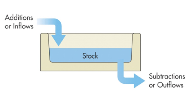
Flows are simply the amounts per period yielded by an asset, or some other thing that happens over time, like investment or depreciation. Stocks are the corresponding total value of an asset at a particular time. Flows have a “time signature,” i.e. rent per month, income per year. Stocks do not: value, or wealth, period, full stop. Stock and flow variables are often related; a bathtub is often used as a useful analogy (Exhibit 1).
Sometimes there’s more than one flow associated with the stock. One particularly relevant real estate example comes from measuring Q rather than P. The stock of real estate is built by two flows, gross investment (how much new space we put in place each year), less economic depreciation (periodic losses from a physically wasting asset). The quickest way to imprint on the difference between flows and stocks is to ponder some other familiar examples:
| Income, GDP | ↔ | Wealth |
| Dividends | ↔ | Stock Price |
| Births, Deaths, Immigration | ↔ | Population |
| Income Statement | ↔ | Balance Sheet |
| Rent | ↔ | Property Value |
Measuring Housing Prices, Rents and Values: Some Details
Next let’s clear up some confusion about terminology. The starting point for confusion is this: what we call the price of housing in common parlance isn’t really a price, except under very strong and usually unreasonable assumptions. It’s another case of “if you are not confused you’re not yet thinking clearly.” Consider Exhibit 2, which presents economists’ terminology, compared to common parlance.
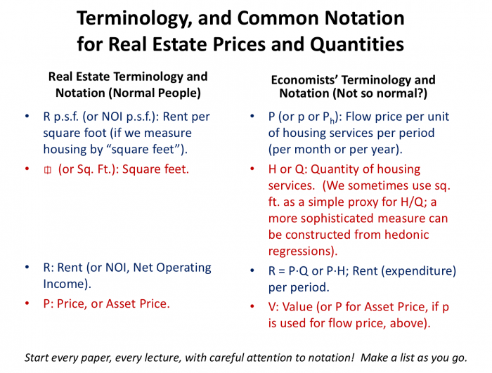
A true price is an amount, usually in dollars (though sometimes expressed in terms of some numeraire good) required to obtain, or the amount received for, a unit of the good or service. Exhibit 2 reminds us that rents, as such, aren’t prices. They are expenditures, or the product of the flow price per unit of housing services, and the quantity of housing services. Values, or asset prices, are the present value of rents. Alternatively, values are the stock price per unit of housing services, times the quantity of housing services delivered by the unit.
Housing services are multidimensional. Many studies of characteristic prices of housing that models such relationships use 20 or more separate variables; 40 or 50 are not unheard of. Nevertheless, often in a housing economics class I simplify the quantity of housing to “square feet,” asking students to imagine that everything else – baths, bedrooms, kitchen, neighborhood and location and so forth – are identical across units. Then square footage stands in for the quantity of housing services; and rent per square foot is in this special case a true flow price. Value per square foot is a true stock price.
Once we move on from a simple classroom exercise to the real world, an obvious question arises. How can we measure the quantity of housing services when quantity is multidimensional, instead of a single measure like square footage? The methods we discussed below, particularly hedonic models and repeat sales techniques, are generally the best methods to recover true prices and, in the case of hedonic models, direct estimates of the quantity of housing services.
Exhibit 2 includes some common notation used in economics publications. Unfortunately, economic notation is not completely standardized so the Exhibit is merely a guide. If you are reading an economics article containing such shorthand, do what I do: make a first pass through the article and on a sheet of paper carefully write out the definition of every symbol used in that paper. Then go back and start reading again with this dictionary in hand.
Even economists misuse terms. I try to remember to say “value” or “asset price,” not simply “price,”
when I mean the value of a unit. I try to say “price” when I’ve somehow controlled for the quantity of housing services produced by a unit. But sometimes I fail, and revert to common parlance, especially in casual conversation.
There is a large and ever-growing number of the sources of housing price data out there, including government sources such as Census, Bureau of Labor Statistics (BLS), Bureau of Economic Analysis (BEA), the Department of Housing and Urban Development (HUD), and the Federal Housing Finance Agency (FHFA). Private sources include the National Association of Realtors, CoreLogic Case-Shiller, and Zillow. There too many academics constructing these price indexes to list; nevertheless, I will shamelessly mention some of my own work with colleagues including Jim Follain, Larry Ozanne, and Tom Thibodeau. Our own Morris Davis is undertaking some of the most interesting current research, estimating housing prices for every census tract in the country.
To make sense of the large number of price measures available, we need a basic taxonomy, based on techniques for constructing such indices. Exhibit 3 lists six general methods of measuring or estimating housing prices. We will discuss each method briefly in turn.
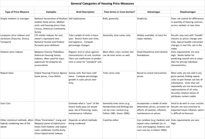
The first type of measure is based on simple medians or averages. The most commonly used measures of this type include median sales prices for existing housing published by the National Association of Realtors (NAR) and Census Bureau median house values and rents. The method is, in general, self-explanatory. Find a sample of housing transactions or appraisals, and compute the mean or the median. Sometimes, other simple statistics are calculated, such as the first quartile or the third quartile, or some other percentile-based measure, as in Malpezzi and Green (1996). HUD’s Fair Market Rents (FMRs), used as housing subsidy benchmarks, are very loosely the 40th percentile of multifamily rents for units meeting basic quality standards, in a given county (for many earlier years, in a given metropolitan area).
The median is usually preferred to the mean, since the distribution of rents and values is usually skewed right by a relatively small number of very expensive units, and there are rarely any negative rents or sales prices; medians give a better measure of central tendency under those conditions. A big advantage of this type of measure is its simplicity, and the fact that comparisons over time and across markets are possible. The biggest disadvantage is that this type of measure does not usually control for differences in quantity of housing services, across markets or over time.
NAR median home price data is available quarterly for about 100 metropolitan areas. They are limited to single-family units, as reported from multiple listing service databases. Alternative median housing “prices” (loosely speaking) are decennial Census median rents and values. In the past, these have the disadvantage of only being available in Census years, but now that the decennial Census is augmented by the American Community Survey, these measures are available more frequently. Both the older decennial Census medians, and the ACS data that have superseded them, are available by state, county, and metropolitan area, and even finer breakdowns through American Factfinder.
Another difference is that Census and ACS data are medians of all units, not just recent sales. They rely on owner self-reported appraisals of value. Studies like Follain and Malpezzi, and Goodman and Ittner, find that these self-appraisals have large variances, but surprisingly modest systematic biases when prices are reasonably stable. Thus self-appraisals are not a precise guide to the market value of an individual unit, but when medians are computed for a reasonably sized sample, positive and negative errors tend to cancel and provide a reasonable, if somewhat biased, estimate.
The direction of the bias is not consistent. The most recent research on self-appraisal biases during the recent boom and bust by Davis and Quentin shows, perhaps unsurprisingly, that homeowners who stay in place tend to underestimate the increase in value of their houses during the boom, and understate the decline in the value of their houses during the bust. Put another way, in the long run these homeowners are perhaps more tethered to fundamentals than a temporarily crazed market.
The second type of measure mentioned in Exhibit 3 is the Laspeyres price index, and its cousins Paasche, Divisia, chain and Tornquist indexes. We discussed these briefly in the previous blog on prices, and in more detail in online class notes. The best known example is the CPI, which attempts to measure the overall cost of living. Laspeyres indexes are constructed as follows: (1) take a sample of units in some base year; (2) revisit them over time, and appraise; and (3) compute percentage changes. More formally, Laspeyres indexes are constructed as:
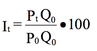
where I is the index, P is the price per unit of housing services, Q is the quantity of housing, and subscripts denote time. Time, 0, is the base year or period, and time, t, is any year, forward (positive t) or backward (negative t). Thus the index is just the ratio of what is spent in time t to what’s spent in time 0, holding constant the “bundle,” or set of goods, purchased in time 0. The variations on the Laspeyres theme represented by its “cousins” have to do with how often the bundle changes and some other technical are of interest but would take us too far afield today.
Hedonic price models provide one way to decompose expenditures on housing into measurable prices and quantities so that rents for different dwellings or for identical dwellings in different places can be predicted and compared. A hedonic equation is a regression of expenditures (rents or values) on housing characteristics, and is explained in some detail in Malpezzi (2003). The independent variables represent the individual characteristics of the dwelling, and the regression coefficients may be transferred into estimates of the implicit prices of these characteristics. The results provide us with estimated prices for housing characteristics, and we can then compare two dwellings by using these prices as weights. For example, the estimated price for a variable measuring number of rooms indicates the change in value or rent associated with the addition or deletion of one room. It tells us in a dollar and cents way how much “more house” is provided by a dwelling with an extra room.
A hedonic price index is in fact a “big data” (or sometimes “medium data”) approach that extends the same basic framework used by a residential appraiser who estimates the value per unit by the method of comparable sales. In the method of comparable sales appraisers rely on recent transactions; but since no two housing units are identical, it’s rare to find a recent transaction or “comp” that is exactly the same in an a nearly identical location as the subject property. Appraisers therefore apply “adjustment factors.” For example if a “comp” sale has three bathrooms and the subject property has two, the appraiser subtracts her estimate of the price of a bathroom from the comparable’s sale price to estimate the value of the subject property. Hedonic regression coefficients in effect give us an entire set of estimates of these adjustment factors for a large set of characteristics, and the model automates the process of pricing a unit.
Once we have estimated the implicit prices of measurable housing characteristics in each market, we can use them for a number of purposes. We can select a standard set of characteristics, or bundle, and price a dwelling meeting these specifications in each market. In this manner we can construct price indexes for housing of constant quality across markets. In a similar fashion we can use the results from a particular market’s regression to estimate how prices of identical dwellings vary with location within a single market (e.g., with distance from the city center) or even to decompose the differences in rent or house values into price and quantity differences.
Repeat sales indexes are estimated by analyzing data from units that have sold at least twice. Such data use regression models that allow us to annualize the percentage growth in sales prices over time. These are time-series indexes in their pure form. They do not provide information on the value of individual house characteristics, or on price levels, only changes. They have the advantage of being based on actual transaction prices, and in principle allow us to sidestep the problem of collecting data on a large number of characteristics. However, units that sell repeatedly are not necessarily representative of all units. Sometimes it’s difficult to tell whether a unit retains the same characteristics across time. For example, remodeling could change a house’s characteristics. And repeat sales models need to be adjusted for physical depreciation of units.
Finally, hybrid indexes combine elements of two or more methods into one index. These could be time series, cross section, or both. For example, we can combine hedonic and repeat sales methods, or hedonic prices and user cost. One type of hybrid model, represented by Quigley (1999), “stacks” repeat sales and hedonic models, and then estimates the two models imposing a constraint that estimated price changes over time are equal in both models. In effect, such methods are weighted averages of the hedonic and repeat sales, and have the advantage of making use of all available information. Another type of hybrid index, as in Malpezzi (1999), combines hedonics, which can estimate place to place differences in levels, with repeat sales, which can only estimate price changes. A set of hedonic prices is used for a baseline year to set levels in different states or metropolitan areas, and then repeat sales are used to estimate levels forward and backward from the benchmark date.
The idea behind user cost is simple, although implementation can be complex. A user cost model aims to determine what a “user” of the house really pays (or would pay), net of financing, taxes, maintenance, inflation, and so on. User cost measures are most often time series but can be cross section. User cost incorporates a model of what actually determines prices, and accounts for the effects of taxation, inflation, and maintenance on prices.
The user cost of housing capital is based on a theory of long-run determination of equilibrium rents (of housing and of other capital). User cost is the cost to use a unit of housing capital each period. For a renter, user cost is the rent he or she pays. For owners of housing capital (landlords and homeowners) it’s more complicated. It’s not especially difficult but it takes a number of steps. User cost is, in the end, a way of building up capitalization rates, i.e. the relationship between stock and flow prices. It’s an important subject, and rather than take a long digression from direct examination of rents and values here, we will devote a separate blog post to user cost and capitalization rates in due course.
Rents – Another Look
Of course this is not our first look at rents in the Rutgers Real Estate Blog. In my first post, on April 13, we examined housing affordability in New Jersey and the Tri-state Area. Compared to other states and the District of Columbia we found that rent burdens (rent-to-income ratios, or budget shares), fell as household incomes rose. This is consistent with housing’s status as a necessity. We found New Jersey had the fifth highest median rents among the 51 states and D.C., with New York and Connecticut close behind. New Jersey’s high rents were partially offset on average by high incomes; but this masked issues with the bottom of the market. New Jersey ranked fourth in the nation (#1 is the worst!) with 47 percent of Very Low Income households (incomes below 50 percent of area median income) reporting that housing consumed more than half their household budget.
On April 29 we examined rent control in metropolitan areas, including a number in the Tri-state Area, and found little prima facie evidence that such controls were effective in reducing rent burdens. Similarly on May 11 we examined inclusionary zoning, and found little positive effect of such programs on rental affordability.
Going beyond these snapshots of state and metropolitan rents and budget shares, in his April 25 post Morris Davis focused on New Jersey and a finer level of geography ZIP Codes and over 23 years. Morris showed that while New Jersey showed very volatile asset prices, rental yields or the rent to price ratios were generally declining over time.
In her post “Blue Skies for Consumers … Clouds for the Fed?, Dr. Coronado already makes the key point that the rent changes we examine today are much “smoother,” less volatile than changes in the asset prices we will examine in two weeks.
Rents in the Consumer Price Index
Now let’s examine the CPI for rent directly. Exhibit 4 presents the rent of principal residences (i.e. for renters) back to 1947, deflated by the CPI after removing all shelter elements. We would prefer seasonally adjusted, data but BLS only provides consistent seasonally adjusted series back to 1981.
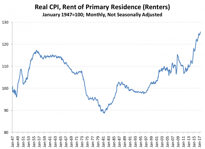
As you already know (Dr. Coronado showed this using some alternative data), asset prices have been much more volatile than rents. We will discuss further in our forthcoming post on asset prices. Over the very long run, over the 70 years of data we see here the real price of housing according to the official BLS CPI grew only 5 percent, or 0.3 percent per year. From the peak in 1956 to a trough in 1981, rents apparently fell by 24 percent, or 1 percent per annum. From that trough in 1981 to the recent and still rising peak, real rents rose by 40 percent, or 1.4 percent per annum.
The long decline in rents between 1956 and the early 80s may be partly due to shortcomings of the data. Until 1985 the rental CPI had a serious problem in the treatment of units in transition between tenants. In brief, when units turned over, they dropped out of the sample. However, it’s during the turnover process that significant rent increases often take place. Ted Crone, Leonard Nakamura and Richard Voith constructed an alternative to the official CPI that estimated the effects of this shortcoming, and their key results are displayed in Exhibit 5.
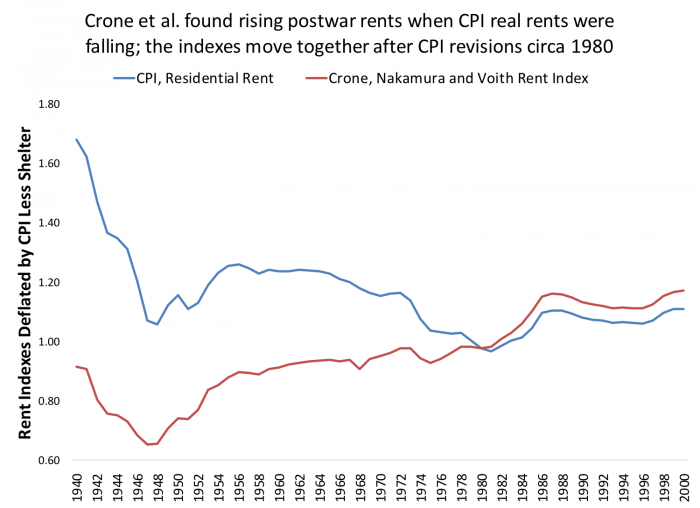
Taking Crone et al.’s corrections at face value, as their article’s title emphasizes, the official CPI showed a long decline in real rents over the postwar period, at least until the 1980s. Their alternative measure shows a sharp decline during the war (partly attributable to wartime rent controls) and a sharp postwar correction as controls were removed from most markets (except New York City, and some New Jersey and California markets, as we discussed earlier). The official index then slowly declines from the mid-1950s until 1981, while the Crone et al. corrections show a slow increase over that same period.
Since a number of improvements in the CPI sample and construction methods over the past 40 years, the two indexes now track each other quite closely.
Exhibit 6 presents our last look, for today, at rents, focusing on the improved data BLS has worked diligently to provide over the past 35 years.
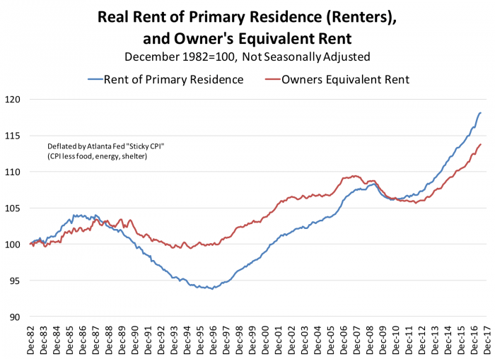
Exhibit 6 presents two rent indexes, one for renters, and one for owners. To understand why we estimate a rent index for owners, it’s useful to examine a very brief and partial history of the housing CPI.
The CPI began in 1913. Initially coverage varied between quarterly, semiannual and monthly indexes. Initially rents were used to proxy homeowner cost as well as renters. In 1947, a regular monthly CPI for housing began publication. In the 1950s, concerned that then still widespread rent controls were biasing housing inflation downward, BLS shifted to the “asset price” approach for homeowners. Homeowner housing prices were estimated as a combination of each period’s purchase price, mortgage interest, property taxes insurance and maintenance and repair costs.
Concerned soon developed it as the asset price approach introduced its own biases, in no small part because of the implicit assumption that every homeowner replaced every period. Another concern was that the asset price method confused housing consumption and housing investment motives by households, while the CPI is all about consumption. So in 1985 the asset price approach for homeowners was replaced by owners’ equivalent rent (OER). OER is BLS’s estimate of a rental index for units that are representative of the owner-occupied stock in terms of structure, quality and location.
BLS provides the OER data back to December 1982. Exhibit 6 compares the rent of principal residences for renters to the owner equivalent rent directly, for the 35 years for which we have data. In Exhibit 6 we are able to present seasonally adjusted data, and also deflate by a smoother base index, the Atlanta Fed’s so-called “sticky CPI,” that pulls out not only shelter, but also the volatile yet trend-reverting components of food and energy.
We can see that owner equivalent rent follows the same cycles as the rent to primary residence, but is much less volatile. Real rents for renters have increased by 0.5 percent per annum since end 1982, but a much higher 1.5 percent since October 2010. Real imputed rents for homeowners grew by 0.4 percent since 1982, and 1.1 percent since 2010.
Overall, when we look at the national rental CPI, real rent increases are very modest in the very long run, consistent with an elastic rental market. Over the past 7 years we’ve seen a much more substantial runup in rents. Based on past performance, we can expect rent growth to moderate and get back to background inflation or below; but it’s difficult to forecast just when such a turn will occur.
Our Bottom Line
There’s a lot of house price data out there but of varying quality. We identified the broad categories of housing price measures and provided a very brief introduction to each. Previous Post we already provided snapshots of rent and rent to income by state and by Metropolitan area. Here we examine imminent rents in time series from the consumer price index. Consistent with previous posts of shorter run data by Julia Coronado and Morris Davis, rents increase slowly – the recent run-up suggests there are important downward biases in the official BLS measure.
Selected Data Sources
The Census Bureau’s Web site is the mother of all data sites.
American Factfinder is a powerful if somewhat tricky front end to pull together a wide range of Census and other data by varying geographies and dates.
iPUMS is a site where you can download a ton of historical data from previous Censuses and other sources.
The Bureau of Labor Statistics is the home of the CPI and a load of other price, wage and economic data.
The Federal Reserve Bank of St Louis maintains FRED, a terrific and easy to use site to find a huge amount of economic data, including a lot of the price indexes we discuss here.
CoreLogic is now the home of the Case Shiller repeat sales housing price indexes.
HUD User is the home of a lot of useful data, including American Housing Survey data, and the Fair Market Rents described above.
The National Association of Realtors is the source of median house prices.
The Federal Housing Finance Agency is a source of a number of repeat sales price indexes.
Zillow provides datasets for research purposes.
References, and Further Reading
Abraham, Jesse M, and William S Schauman. “New Evidence on Home Prices from Freddie Mac Repeat Sales.” Real Estate Economics 19, no. 3 (1991): 333-52.
Bureau of Labor Statistics. “BLS Handbook of Methods.” US Department of Labor (1997).
Case, Brad, Henry O. Pollakowski, and Susan M. Wachter. “On Choosing among House Price Index Methodologies.” Real Estate Economics 19, no. 3 (1991): 286-307.
Crone, Theodore M, Leonard I Nakamura, and Richard Voith. “Rents Have Been Rising, Not Falling, in the Postwar Period.” The Review of Economics and Statistics 92, no. 3 (2010): 628-42.
Davis, Morris A, Stephen D Oliner, and Edward J Pinto. “House Prices and Land Prices under the Microscope: A Property-Level Analysis for the Washington, Dc Area.” Working Paper, American Enterprise Institute, 2014.
Davis, Morris A, and Erwan Quintin. “On the Nature of Self‐Assessed House Prices.” Real Estate Economics (2016).
Follain, James R., Jr., and Stephen Malpezzi. “Are Occupants Accurate Appraisers?” Review of Public Data Use 9, no. 1 (April 1981): 47-55.
Goodman, John L, and John B Ittner. “The Accuracy of Home Owners’ Estimates of House Value.” Journal of Housing Economics 2, no. 4 (1992): 339-57.
Green, Richard K., and Stephen Malpezzi. A Primer on U.S. Housing Markets and Housing Policy. American Real Estate and Urban Economics Association Monograph Series. Washington, D.C.: Urban Institute Press, 2003.
Greenlees, John S, and Robert B McClelland. “Addressing Misconceptions About the Consumer Price Index.” Monthly Labor Review 131 (2008): 3.
Hamilton, James D. “Understanding Crude Oil Prices.” The Energy Journal 30, no. 2 (2009): 179-207.
Liang, Yongping and Stephen Malpezzi. “Recent Price and Quantity Volatility in Metropolitan Housing Markets: A First Look.” James A. Graaskamp Center for Real Estate Working Paper. Madison, WI: University of Wisconsin, 2017.
Malpezzi, Stephen. “Hedonic Pricing Models: A Selective and Applied Review.” In Housing Economics and Public Policy: Essays in Honour of Duncan Maclennan, edited by Tony O. O’Sullivan and Kenneth Gibb, 67-89. Malden, Mass. and Carlton, Australia: Blackwell Science, 2003.
———. “A Simple Error Correction Model of House Prices.” Journal of Housing Economics 8, no. 1 (March 1999): 27-62.
Malpezzi, Stephen, Gregory H. Chun, and Richard K. Green. “New Place-to-Place Housing Price Indexes for U.S. Metropolitan Areas, and Their Determinants.” Real Estate Economics 26, no. 2 (Summer 1998): 235-74.
Malpezzi, Stephen, and Richard K. Green. “What Has Happened to the Bottom of the Us Housing Market?” Urban Studies 33, no. 10 (December 1996): 1807-20.
Malpezzi, Stephen, Larry Ozanne, and Thomas Thibodeau. “Characteristic Prices of Housing in Fifty-Nine Metropolitan Areas.” Research Report, The Urban Institute, Washington, DC (1980).
McCarthy, Jonathan, and Richard W Peach. “The Measurement of Rent Inflation.” (2010).
Miller, Norman G. Jr., and Sergey Markosyan. “The Academic Roots and Evolution of Real Estate Appraisal.” Appraisal Journal 71, no. 2 (2003).
Moulton, Brent R. “Issues in Measuring Price Changes for Rent of Shelter.” Paper presented at the Conference on Service Sector Productivity and the Productivity Paradox, 1997.
Poole, Robert, Frank Ptacek, and Randal Verbrugge. “Treatment of Owner-Occupied Housing in the Cpi.” Federal Economic Statistics Advisory Committee (FESAC) on December 9 (2005): 2005.
Ptacek, Frank, and Robert M Baskin. “Revision of the CPI Housing Sample and Estimators.” Monthly Lab. Rev. 119 (1996): 31.
Quigley, John M. “A Simple Hybrid Model for Estimating Real Estate Price Indexes.” Journal of Housing Economics 4, no. 1 (1995): 1-12.
Wang, Ferdinand T, and Peter M Zorn. “Estimating House Price Growth with Repeat Sales Data: What’s the Aim of the Game?”. Journal of Housing Economics 6, no. 2 (1997): 93-118.