
Housing market regulation part II: Costs and benefits
In previous posts, we’ve argued that the twin pillars of effective housing policy are housing vouchers on the demand side – for citizens we decide need assistance with housing costs, given their age, disabilities or poverty – and regulatory reform on the supply side. Supply-side regulatory reforms, of course, will often prove salutary for the entire market – for low, middle, and upper income households alike.
Our last post, introducing supply-side regulatory issues, provided: motivation for regulation of real estate markets, namely a discussion of market (and government) failure; a brief history of planning, zoning, and other regulations; and an initial examination of different types of real estate regulation. We then developed a simple effective toolkit for rigorous study of the costs and benefits of regulations.
Today’s post dives deeper into a range of empirical topics: measuring regulation, and another important supply determinant, namely physical geography; and why and how communities choose their regulatory environments. Then we present an example of cost-benefit analysis that provides some empirical results on how regulation affects housing market outcomes: prices and quantities of housing; benefits to housing consumers and their neighbors; and possible spillovers to the broader economy.
Finally, in April, our third post on this broad and important topic will draw upon results from this and previous posts to develop recipes for reform, to deliver fairer and more effective real estate regulation, and, even more importantly, fairer and more effective real estate market outcomes.
Measuring Regulation
Broadly, two kinds of empirical studies provide the evidence required for improved policies: (1) detailed cost case studies of the costs and benefits of regulations in individual markets or projects; and (2) comparative studies of the effects of regulatory measures across markets. Given space constraints, today’s post will focus on Type 2, cross-market regulatory comparisons, although will also draw on lessons from case studies as needed.
In a blog post our review of research is necessarily very selective. Many dozens of studies have been carried out in both the case study vein as well as cross-market studies. A detailed literature review isn’t feasible here, but in addition to the short list of references at the end of the post, see also the many references contained within, and especially excellent detailed surveys found in Fischel (2015) and Gyourko and Malloy (2015).
To begin, we’ll focus on a regulatory measure from Malpezzi (1996). That study constructed a regulatory index based on a 1989 survey of hundreds of planning directors in 60 large metropolitan areas by a team from Wharton. Linneman and Summers 1990 and Buist 1991 document the original data collection. From that survey we first constructed seven subcomponents each on a scale of 1 to 5, with 1 representing the least restrictive value of the questionnaire element and 5 the most stringent. These subcomponents measure: (1) the change in approval time (zoning and subdivision) for single family projects between 1983 and 1988; (2) the estimated number of months between application for rezoning and issuance of permit for a residential subdivision less than 50 units; (3) a similar variable, but based on the time for single family subdivision greater than 50 units; (4) a qualitative assessment of how the acreage of land zoned for single family compares to demand; (5) the amount of acreage of land zoned for multifamily compared to demand for multifamily; (6) the percentage of zoning changes approved; (7) the adequacy of infrastructure (roads and sewers) compared with demand. Testing arts-and-craftsy statistical methods for combining these elements into an index demonstrated that a simple linear scale was just as good as more complex techniques like principal components. (Don’t ask.) We named the linear scale REGTEST. The lowest possible score is 7 and the highest 35. Chicago had the lowest actual value of REGTEST, 13, while San Francisco and Honolulu had values of 29.
Exhibit 1 presents a simple two-way plot of the metropolitan areas of home values by the REGTEST index. Specifically, the vertical axis measures median house value from the 2010 Census, adjusted using the GDP deflator to $2017. The horizontal axis is the linear index REGTEST. Each metropolitan area or division is represented by a short mnemonic code. Four observations represent our region and are highlighted in red: the New York, Philadelphia and Hartford metropolitan areas, and the Newark metropolitan division.
Note that, as promised, the metropolitan-level analysis gives us a richer look at the relationship between regulation and housing costs than the state level data we presented in Exhibit 1 of the first post on regulation.
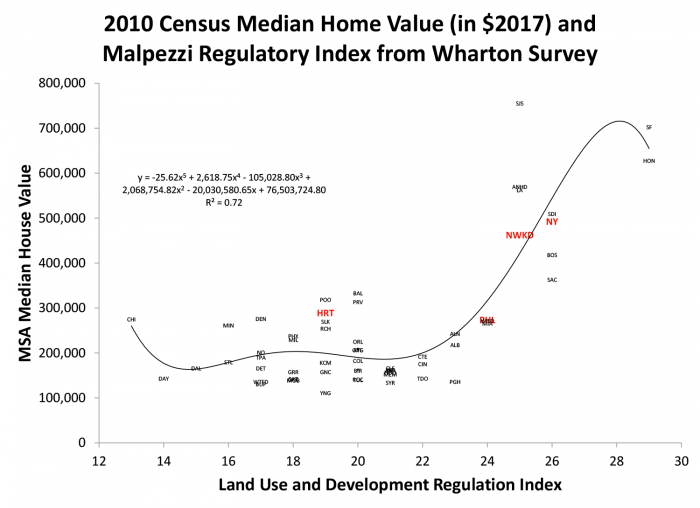
We fit a regression line through the 50 observations, but it’s a flexible power function that allows us to smooth the data without being too restrictive. Chicago was already flagged as the least restrictive value of REGTEST with a value of 13; a bit of a surprise, but like Steve Harvey we go with what the survey says. While Chicago drives the regression line up a bit, for much of the data, from a regulatory value of 14 (Dayton) to about 24 (Philadelphia and Miami) there isn’t much of a trend in house values. Of course there is variation around those trends (moving averages). For example in the middle of the REGTEST index are metro areas like Portland, Baltimore, Providence and Hartford with median house values around $300,000, while at the same level of regulation Youngstown barely breaks $100,000. That’s no surprise given the wide variation of other variables that can affect how home values including demographics, income and geographical constraints. But from a REGTEST value of about 24 up through the peak value of 29 there is a very steep increase in home values associated with increased regulatory stringency. Newark and New York are among those in the more stringently regulated part of the data although they are less restrictive than San Francisco and Honolulu and much less expensive. San Jose comes in with a similar REGTEST score to Newark but a much higher home value; unsurprising given the much higher demand pressures in that metropolitan area.
REGTEST, and all other such indexes, are constructed from a reduced information set. There are literally hundreds of individual regulations and possible candidate measures. The maintained hypothesis of such studies is that there is some correlation between included and excluded measures, and the measures presented are a latent variable for some unobservable “regulation.” Coefficients of such models should not be taken literally as the exact partial effects of individual components. But studies including Gyourko, Saiz and Summers demonstrate that there is substantial correlation among individual regulations; markets with restrictive zoning tend to have more stringent building codes and subdivision regulations; and vice versa. Thus, despite their shortcomings, such indexes can be a reasonable guide to which markets are broadly more stringently regulated.
Measuring Physical Geography
It’s not just regulation that constrains housing supply in some markets – physical geography matters, too. Early cross-market studies, including my own, often used some measure of land area lost to large bodies of water (oceans and the Great Lakes). These were sometimes measured simply as dummy variables, or by using a protractor to roughly measure the arcs of the circle lost to these bodies of water. A few studies also examine whether there were constraints to growth by adjoining metropolitan areas and/or national parks and military reservations. But consider Exhibit 3 (licensed from iStock), a readily recognizable aerial photo of San Francisco, highlighting the mountains that remind us there are other physical barriers to development besides bodies of water.

Several studies have used GIS and satellite data from the U.S. Geographic Service to develop much improved summary indexes of geographic constraint. To date the best comprehensive measures have been provided by Albert Saiz. Saiz uses USGS data and GIS techniques to measure the amount of land lost both to large bodies of water and wetlands, as well as land areas with slopes greater than 15 percent, a reasonable threshold for development.
The metro areas Saiz chose for his measures of geography match up well with the regulatory measures in Gyourko, Saiz and Summers (2008). The latter study extended and updated the original 1989 Wharton Survey used to produce REGTEST, described above. Since the new Wharton measure matches up very well with Saiz’s geographical constraints, Exhibit 3 presents the correlation between these two. Once again several markets of local interest are highlighted in red: the Hartford and New Haven metropolitan areas, and the New York and Newark metropolitan divisions.
The new Wharton regulatory measure used the aforementioned principal components method to aggregate data, rather than the simpler linear technique. Principal components yield a measure which is centered upon zero for an “average” regulatory environment. Assuming a normal distribution, a value of one is about a standard deviation away from the average metro area; a value of two, two standard deviations. A positive value means a more restrictive environment, and a negative value means a less restrictive environment. On the far right of Exhibit 3, for example, about 80 percent of the land around Oxnard, CA is constrained, while about 75 percent of the land around New Orleans is constrained. But turning our attention to the vertical axis, New Orleans has one of the least restrictive regulatory environments and Oxnard one of the most restrictive. At the other extreme almost all the land in Fort Wayne Indiana and Wichita Kansas is developable, and they have a very permissive regulatory environment. Providence is not too far from another “corner” in the Exhibit – about 85 percent developable land, but with a very restrictive environment.
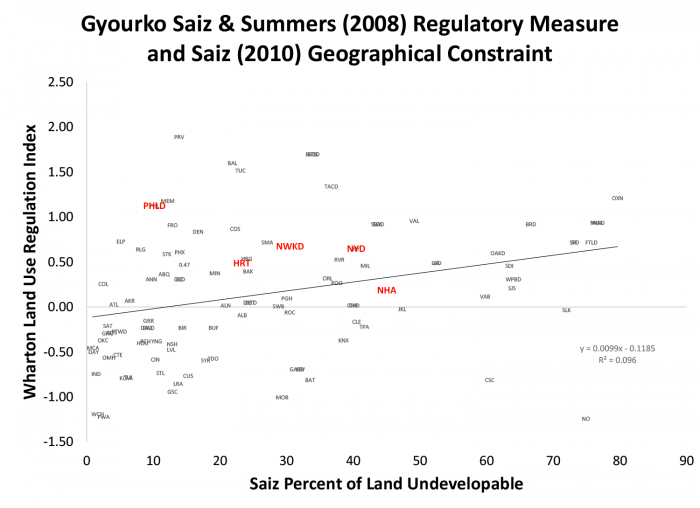
In our region, New Haven is about average and our other three regional data points (Hartford, Newark and New York) are somewhat above average in terms of regulatory restrictiveness according to the newer Wharton regulatory indexes. They are also above average in terms of geographic constraint with between 20 and 45 percent of their land undevelopable, according to Saiz’s measure.
Overall, while the relationship is not terribly tight, Exhibit 3 suggests there is some tendency for more geographically constrained locations to have more stringent land use and development regulations. Next, we’ll explore some other reasons some locations have more stringent land use and development regulations than others.
Choice of Regulatory Environments
In our previous post we showed that land use and development regulations have a long history, about as long as the history of cities if we take a long view; and since the 1920s if we focus on American-style zoning. But starting around the 1970s, as Fischel and others explain, some cities began to ramp up the restrictiveness of the regulatory environment.
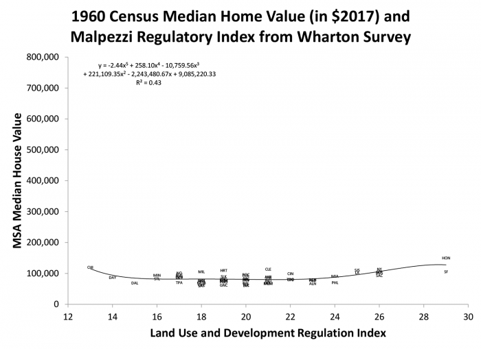
The world did not always look like Exhibit 1. Exhibit 4 is similar to Exhibit 1, using the same regulatory index on the horizontal axis, but using 1960 Census median home values (in constant 2017 dollars) on the vertical axis. Notice how much lower and flatter the data are. Some of the difference between 1960 and 2010 home values is due to the improved quality and larger size of houses. But back-of-the-envelope calculations, using the rate of replacement of old housing stock with new, the growing size of new units, and the rate of depreciation of the old stock, confirms that the majority of the difference between Exhibit 4 and Exhibit 1 is due to differences in prices rather than quantities (size and quality of unit).
We constructed charts like Exhibit 4 for each Census year, and it becomes apparent that there is a breakpoint circa 1970 where home values start to rise a lot faster in the metro areas that later had more stringent regulations, leading to the “hockey stick” regression line Exhibit 1. Another way to look at this phenomenon is to simply examine the relationship between the regulatory environment in 1990 and the prior growth of real house values in the preceding 30 years, in Exhibit 5. Here the pattern is clear – cities with faster home value growth over 30 years ended up with more restrictive regulation at the end of the period.
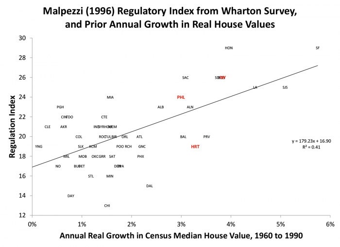
Taken together, the data in Exhibits 1, 4 and 5 are consistent with William Fischel’s so-called “Homevoter Hypothesis,” which starts with the premise that risk-averse and loss-averse homeowners have stronger incentives to limit competing development when their initial home values are high. In a dynamic setting, a shock which increases home values gives rise to demand for more stringent regulation, which in turn further increases home values, in a sort of spiral. This phenomenon is consistent with what we see in the pattern of home prices over time in the California, New York and Hawaiian markets. The framework suggests that recent increases in home prices since 2009 could fuel additional demand for more stringent regulations. Of course, there can be limits, as at some point extremely high home values can reduce in-migration, household formation and economic growth.
Fischel’s model is now widely accepted, but the Homevoter Hypothesis and other explanations are not mutually exclusive. Other phenomena can affect both the demand for the supply of regulation; some can be integrated into the Homevoter model.
Why exactly would it be that additional development threatened existing home values? Partly it can be a simple matter of supply and demand for the number of housing units within a market, but there are other channels that can be at work. One much discussed by Fischel and other scholars are fiscal externalities. These can be especially important in a system of Balkanized local governments as are found in many U.S. metropolitan areas. Consider a given municipality and/or school district with a large tax base from commercial property, and few residents, especially few residents with public school students. The assumption would be such a municipality would have a surplus from substantial tax revenue but relatively few demands on local public services. Suppose the municipality/school district next door has little commercial property but many moderate income households living in apartments, commuting to the jobs in the adjoining municipality. The first municipality, it is argued, will accrue a fiscal surplus while the second municipality will spend a lot more on schools, without recouping substantial property taxes from commercial real estate. Cooley and LaCivita (1982) formalize this with a theoretical model of the demand for controls driven by such fiscal externalities and congestion. Lenon, Chattopadhyay and Heffley (1996) study Connecticut townships and find that each town’s zoning, taxing and spending policies are strongly related to those of neighboring towns.
Another motivation for homeowner resistance to development is that some homeowners may have an aversion to low-income and/or minority populations, whether for the fiscal reasons just mentioned, or simple prejudice. Rolleston’s study of northeastern New Jersey finds the restrictiveness of residential zoning is positively related to the relative fiscal position of a locality, and negatively related to the size of minority population. Gin and Sandy use zip code level voting data from San Diego and find larger minority populations (and, surprisingly, higher incomes) weaken support for controls.
A related question is whether “affordable housing” affects nearby property values. Many (potential) neighbors of low-cost developments are concerned that “affordable” developments will lower nearby property values. Research suggests otherwise. A dozen careful studies (including one of Madison and Milwaukee by Green, Malpezzi and Seah) fail to find much effect. That does not mean a badly designed or located project could never reduce values, but that in practice we seem to site projects appropriately.
Regulation and Real Estate Market Outcomes
Malpezzi (1996) did more than construct some regulatory indexes and produce plots like Exhibit 1. The data were also used to carry out a more complete cost benefit study.
It bears noting that regulations, like other activities, have both costs and benefits. Are planners biased towards benefits? Are economists biased towards costs? We’ll dive more fully into this question in the third installment next month, but for now note that, as we did in the first post, a regulation or a tax that perfectly corrects for a large externality can readily increase housing prices. Thus, showing that regulation increases prices or values is not the end of the story. Like Paul Harvey, we need the rest of the story. Are there corresponding benefits? And how big are these benefits relative to the costs?
Possible sources of costs and benefits were discussed in our first post, and above. They include changes in prices (rents and house values); changes in homeownership rates; traffic congestion, as well as congestion of other public services; changes in racial, ethnic and economic segregation; environmental/neighborhood effects, e.g. rainwater runoff, fire risk etc.; and the aforementioned fiscal effects, changes in tax revenue and local public expenditure.
Armed with data on regulation, physical geography, home values but also rents, incomes, commuting times, measures of neighborhood satisfaction, and homeownership rates, among other data, Malpezzi (1996) estimates a series of simple cross-metro area regression models. Regression models allow us to study relationships among a number of variables, in other words to generalize beyond our simple two-way plots. We can then isolate each affect, what economists call ceteris paribus effects or “holding everything else equal.” We can also use the regression coefficients to simulate policy changes or changes in the economic environment. The full paper and results are available here.
Estimation of the models begins with “reduced form” regressions of prices (rents and house values) against “The Usual Suspects” (income, population and demographics; in levels and rates of change), and our key regulation and physical geography variables. We then estimate similar regressions of several benefit measures against prices, regulation, and other determinants like income and demographics. Specific benefit measures studied include homeownership, reduced segregation, increased neighborhood satisfaction, reduction in commute times.
Key results included the following. For rents and house prices, the “usual suspects” (income, population) worked well; regulation raised rents and asset prices, but raised asset prices much faster than rents. More stringent regulation lowered homeownership rates, primarily through effects on prices. The only “externality” measure that was significantly affected directly by regulation was average commute (congestion).
But we found that regulation affected tenure choice indirectly. This bears a little explanation. Relative rents/asset prices (values) affect tenure choice. Higher rent, ceteris paribus, increases homeownership. Higher values, ceteris paribus, lowers homeownership. Now, our results show that regulation drives up rents and values. But it drives up rents less than values; hence the indirect effect of higher regulation on homeownership is, on balance, negative.
We then used the regression results to simulate changes in regulation. Our main simulation proceeded as follows. Define an arbitrary “lightly regulated” city and a “heavily regulated city;” we defined this change as moving from the first quartile of regulatory indices to the third quartile. Infinitely many other changes can be simulated, but for this specific simulation we find:
- Rents go up by 17%
- Values go up by 51%
- Homeownership rates go down 9 points
- Average commutes go down 3 minutes per day
- No significant effect on segregation or neighborhood
Of course, these results are hardly the final word. Progress in economic research is always incremental, every study that answers two or three questions engenders half a dozen new ones. To give just a few examples… Our regulatory index can be improved, especially if we “endogenize” it, i.e. account for the fact that in reality price and regulation are intertwined. There are many benefit measures that we haven’t tested, including the fiscal measures emphasized in Fischel and much of the rest of the literature. Updating the data, and incorporating the latest regulatory and geographical measures should prove fruitful. But even the simple exercise summarized here gives some of the flavor of what we’ve learned about regulation, and how we go about learning. In fact there’s already been substantial work on these and other questions; we began with Malpezzi (1996) because it was a good paper to illustrate principles. We could do a dozen posts on later studies as our stock of knowledge is increasing.
Final remarks
In this post we’ve had a taste, but only a taste, of what empirical research can tell us about the nexus between regulation and housing market outcomes. Our exploratory data work with two-way plots (confirmed by many other studies, only some of which are cited here) demonstrates that more stringent regulations increase prices and, to at least some extent, these very increases in prices can in turn create pressures for more stringent regulations. Our model found that very stringent regulatory regimes as in California cities yield high costs and little in the way of measured benefits; but we also found that there was a substantial range over which price effects were modest.
We were able to directly examine several markets we think of as our own that we can identify within our sample. Newark and New York City are more stringently regulated than most cities, although not yet at the level of the most stringently regulated California cities or Honolulu. Hartford and Philadelphia are closer to the mainstream of regulatory stringency. We will have more to say about these results, and bring in some others, as well as a more detailed policy discussion, in our third installment on land use and development regulation, in mid-April. Stay tuned!
Sources, and Further Reading
Buist III, Henry. “The Wharton Urban Decentralization Project Database.” University of Pennsylvania, Processed (1991).Cooley, TF, and CJ LaCivita. “A Theory of Growth Controls.” Journal of Urban Economics 12, no. 2 (1982): 129-45.
Fischel, William A. “Do Growth Controls Matter?”. Lincoln Institute of Land Policy, Cambridge Massachusetts (1990).
———. “Externalities and Zoning.” Public Choice 35, no. 1 (1980): 37-43.
———. “Fiscal Zoning and Economists’ Views of the Property Tax.” In Available at SSRN 2281955: Dartmouth College Department of Economics, 2013.
———. “Zoning Rules! The Economics of Land Use Regulation.” Cambridge, MA: Lincoln Institute of Land Policy (2015).
Gin, Alan, and Jonathan Sandy. “Evaluating the Demand for Residential Growth Controls.” Journal of Housing Economics 3, no. 2 (1994): 109-20.
Glaeser, Edward L, Joseph Gyourko, and Raven E Saks. “Why Is Manhattan So Expensive? Regulation and the Rise in Housing Prices.” The Journal of Law and Economics 48, no. 2 (2005): 331-69.
Green, Richard K. “Land Use Regulation and the Price of Housing in a Suburban Wisconsin County.” Journal of Housing Economics 8, no. 2 (1999): 144-59.
Green, Richard K, Stephen Malpezzi, and Kiat-Ying Seah. “Low Income Housing Tax Credit Housing Developments and Property Values.” Madison, WI: The Center for Urban Land Economics Research, The University of Wisconsin (2002).
Gyourko, Joseph, and Raven Molloy. “Regulation and Housing Supply.” In Handbook of Regional and Urban Economics, edited by Gilles Duranton, J Vernon Henderson and William C Strange: Elsevier, 2015.
Gyourko, Joseph, Albert Saiz, and Anita Summers. “A New Measure of the Local Regulatory Environment for Housing Markets: The Wharton Residential Land Use Regulatory Index.” Urban Studies 45, no. 3 (2008): 693.
Lenon, Maryjane, Sajal K Chattopadhyay, and Dennis R Heffley. “Zoning and Fiscal Interdependencies.” The Journal of Real Estate Finance and Economics 12, no. 2 (1996): 221-34.
Linneman, Peter D, and Anita A Summers. “Patterns and Processes of Employment and Population Decentralization in the United States.” Urban change in the United States and Western Europe: Comparative analysis and policy (1999): 89.
Malpezzi, Stephen. “Housing Prices, Externalities, and Regulation in U.S. Metropolitan Areas.” Journal of Housing Research 7, no. 2 (1996): 209-41.
McDonald, John F, and Daniel P McMillen. “Determinants of Suburban Development Controls: A Fischel Expedition.” Urban Studies 41, no. 2 (2004): 341-61.
Mills, Edwin S. “Why Do We Have Urban Density Controls?”. Real Estate Economics 33, no. 3 (2005): 571-86.
Rolleston, Barbara Sherman. “Determinants of Restrictive Suburban Zoning: An Empirical Analysis.” Journal of Urban Economics 21, no. 1 (1987): 1-21.
Saiz, Albert. “The Geographic Determinants of Housing Supply.” The Quarterly Journal of Economics 125, no. 3 (2010): 1253-96.
Xing, Xifang, David Hartzell, and David Godschalk. “Land Use Regulations and Housing Markets in Large Metropolitan Areas.” Journal of Housing Research 15, no. 1 (2004): 55-79.