
Comparing U.S. home mortgage markets, historically and globally
Many of our Rutgers Real Estate blog posts focus on problems in our economy and the real estate markets. We propose fixes to the problems by obtaining stable or faster growth through a fairer system of housing subsidies for those in need or a better allocation of office or industrial space. But if we focus only on problems, it’s not because we’re a bunch of Cassandras. We are very interested in making a good economy better, improving housing and commercial real estate markets that have performed impressively well by most global and historical standards. And true, sometimes we get things disastrously wrong. We’ve got that triple whammy of the 2000s era housing boom and bust, Great Financial Crisis, and Great Recession to explain. Looking for improvements, that’s why are we always picking away, whining about reforming land use and development regulations, improving macroeconomic policies or fixing a broken immigration system. And of course this quest for continuous improvement very much applies to real estate finance.
If sports analogies are permitted, it’s as if we are offering to coach basketball players at Rutgers (or my alma mater LaSalle, or Morris’ Penn, or Julia’s Texas) about how to get to that Villanova or Connecticut level. Any normal gym rat knows the worst player on a mediocre Division I team is a talented and well-trained athlete. But they have to put in more work. Even the greatest players of all time – Lebron, say, or either of the Birds (Sue or Larry) – never stopped working to improve. Michael Jordan [video 1], [video 2] famously failed to make his high school team as a sophomore, which further fueled his work ethic. Maybe that’s a large part of why they became great to begin with? James Bailey was known for his thunderous dunks, Eddie Jordan for his defensive stops, Phil Sellers for his all-around play, but first and foremost, none of these Rutgers’ basketball players were ever satisfied with their performance.
Some aspects of our economy and real estate markets might be “Lebrons,” performing impressively but still capable of improvement. Other aspects, perhaps, more closely resemble the laggards in a middle-school gym class (been there) – not so good at the moment, maybe even terrible. But knowing that with well directed hard work, anyone can improve.
Let’s redirect our attention from basketball to the real point of this essay – mortgages. In May, real estate finance will be one of the themes at our joint conference with Pulte Homes at the New York Stock Exchange. Since mortgage and related financial markets will be a focus, these blog posts will serve as preparation for the meeting. Be ready for the pop quiz on May 15!
Many of the housing finance issues we face are embedded in a particular set of institutions and practices that we have grown used to over time – so familiar that we have difficulty imagining a world without them. The 30 year fixed-rate mortgage? The mortgage interest deduction? Fannie Mae and Freddie Mac? No recourse beyond house equity in default? No prepayment penalties? Ninety-five percent plus loan-to-value ratios? The point is not that we should scrap all this wholesale, but rather that it’s important to understand where these and other particular features of our housing finance system come from, what purpose they serve, and whether other institutions or practices might perform these functions as well or better, in terms of outcomes, cost, and fairness.
One way to evaluate these institutions and practices is to step back from our own particular set and compare ours with the institutions and practices of other places. Since the U.S. housing finance market is in large part a national system (albeit with a lot of local participants), those other places can be countries. And, to complement cross-country analysis, we examine how we did these things in the past. After all, as L.P. Hartley famously opened his novel The Go-Between, “The past is a foreign country. They do things differently there.”
This first of two posts will focus on our mortgage system in historical perspective. A companion post, in a few weeks, will focuses on cross-country comparisons, where we fit in internationally.
Before we tackle the mortgage market, the next section will present a little economic context for our housing finance system. Real GDP per capita will serve as our main indicator of the state of the economy. Then we’ll present some very basic mortgage data focusing on long-run trends in mortgage debt outstanding and mortgage rates. The third section will outline some of the major institutional history. A brief section then examines homeownership and very briefly discusses where taxes and house prices fit into this discussion. The blog concludes with a thumbnail sketch of where we are today, setting the stage for the next blog.
Today’s U.S. Economy in Historical Perspective
There are literally dozens of indicators that could be examined to study the economic context for a mortgage market. To keep the focus of today’s blog on mortgage rates, we will set the stage with only a brief discussion of GDP per capita. Chapter 2 of Davis’ Macroeconomics for MBAs and Masters of Finance is an excellent discussion of a broader range of indicators, including further discussion of the one we consider here. There is no single indicator that tells us everything we need to know about the economy but if forced to pick one for brevity, real GDP per capita is the best choice.
Exhibit 1 presents U.S. real gross domestic product per capita, plotted over time using a logarithmic scale. The data are quarterly. From 1947 to date they are from the Bureau of Economic Analysis, the usual government source. Between 1875 and 1946 the data are from an historical study by Balke and Gordon.
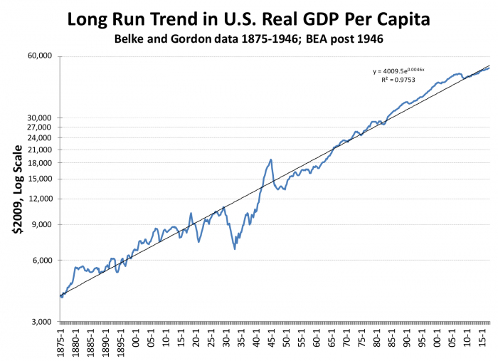
In 1875 real GDP per capita was about $4000 per annum in today’s dollars. Now it’s getting close to $60,000. How rapid a rate of growth is that? A logarithmic scale has a useful property that in a time series, the slope of the line is approximately the percentage change in the variable. The fact that the data lie more or less along a straight line tells us that the very long run rate of growth of real GDP per capita is approximately constant. That rate of growth is just under half a percent per quarter or about 2 percent per year. In the last 15 years or so growth in real GDP per capita has been slower than the long-run average would suggest.
Exhibit 1 also shows the precipitous drop in real GDP per capita associated with the Great Depression and the rapid growth and bounce back, albeit with a significant relapse in the mid-30s. There was also an extremely sharp recession immediately after World War II, but from a peak so high that the 1946 recession is not discussed as much is it perhaps should be.
If you look closely, you can also see growth rates are generally above the long run trend in the expansions of the 80s and 90s. But overall, the hit we took in the Great Recession is significant but nowhere near what we experienced in the 30s.
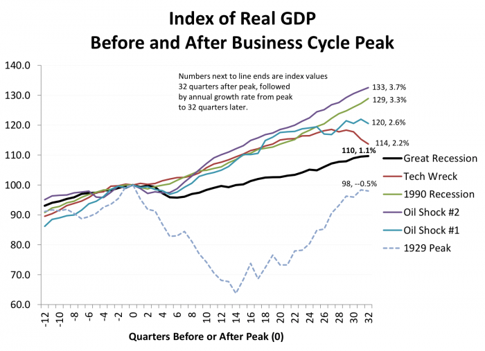
We can get a better look at the latest business cycle using another transformation of our GDP data in Exhibit 2. This is simply a transformation (from dollars to index numbers) of the same data that was used in Exhibit 1, except that we used real GDP this time, not per capita. Thus Exhibit 2 includes the effect of population growth as well. By construction, if we re-did Exhibit 2 with real GDP per capita, all the lines would be a bit flatter, but their relative positions would be preserved.
Specifically, Exhibit 2 presents real index numbers for U.S. GDP around the five most recent business cycles, normalized and centered at their individual peak quarters, presenting 3 years of data before each peak and 8 years afterwards.
The most recent business cycle is represented by the thick black line. Circa July 2006, booming U.S. house prices turned down; on average, prices fell 30 percent in real terms before rebounding in 2012. The declines in more volatile major markets in states like New York, California, Florida and Nevada were substantially larger; Los Angeles prices fell by half, by some measures, and Las Vegas by two-thirds. The impact on mortgage markets and their derivative securities was severe, leading to several traditional bank runs (depositors clamoring for their funds back) as well as a much more severe run on short-term money markets. Among many other notable 2007 events, subprime lenders New Century Financial Corporation and American Home Mortgage filed for bankruptcy, and the largest originator, Countrywide, was downgraded to near-junk bond status on its way to eventual takeover by Bank of America. U.S. subprime problems were already spilling overseas, for example to UK’s Northern Rock. In September 2008 the collapse of Lehman Brothers heralded a massive global financial shock.
On the “real side” of the economy, the U.S. entered recession in December 2007 (Q4 2007 when presenting quarterly data), according to the National Bureau of Economic Research. The recession was the deepest since the 1930s Great Depression, with a 5 percent decline in real GDP. The recovery came in June 2009, but while the post “Great Recession” recovery has been long, it has been shallow, with growth rates roughly half of that normally observed in expansions.
The Great Recession has thus earned its unofficial but widely used moniker. But for perspective, Exhibit 2 also overlays the 1930s era Great Depression (officially, two recessions dated August 1929 to March 1933, and May 1937 to June 1938). Without minimizing the cost of the 5 percent peak-to-trough decline in real GDP in the Great Recession, the corresponding decline in the Depression was about a third, and that from a much lower beginning level, with much less of a social safety net.
Estimating the full cost of the crisis and its aftermath is difficult. Much depends on what counterfactual we assume about the time path of output, employment and so on in the absence of the crisis. This benchmark is, of course, unknowable with any degree of precision. Luttrell, Atkinson and Rosenbaum (2013) estimated the total cost of the Great Financial Crisis on lost U.S. output at somewhere between $6-14 trillion; Ollivaud and Turner estimate that 19 OECD countries that experienced their own financial crises, some of which could be econometrically linked to the U.S., typically lost 5 or 6 percent of GDP. Dullien et al. (2010) found large costs in developing countries as well. While some countries, notably China, avoided a measured contraction at the time, according to the World Bank, global GDP fell between 2008 and 2009, whether measured at market or purchasing power parity exchange rates, the largest of only 3 global contractions in a half century.
Basic Historical Data on the Residential Mortgage Market
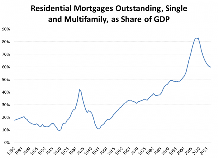
Exhibit 3 presents the most basic quantity data, the amount of residential loans outstanding, single and multifamily combined. Today that quantity stands at about $11 trillion and it peaked in 2008 at about $12 trillion. However, to give a clear picture of how the size of the mortgage market expanded relative to the economy Exhibit 3 presents mortgages outstanding as a share of GDP. (Mortgages outstanding are a stock measure, and GDP is a flow, which we usually prefer not to mix, but it is a conventional way of scaling large numbers like long-term debt).
Circa 1890, the size of the mortgage market was less than 1/5 of GDP. After World War II there was a rapid run up from a low of about 10 percent at the end of the war to 40 percent only six years later. But with the crash and the many defaults (memorialized in the classic Frank Capra movie It’s A Wonderful Life) we were back to 10 percent. At the end of World War II there was a rapid if not completely steady increase from a mortgage market 1/10 of the size of the flow economy to one that peaked at over 80 percent of GDP in 2008, now down to 60 percent.
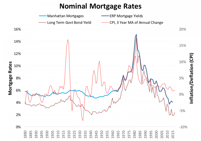
Exhibit 4 presents some long run data on nominal mortgage rates. From 1965 to date these rates are represented by mortgage yields on fixed rate loans from the Economic Report of The President. Prior to 1965 it’s hard to find national data, but Wenzlick provides data on mortgage rates in Manhattan that we can take as at least a crude estimate of rates over time.
Exhibit 4 also includes data on inflation, and on the yields on government bonds as benchmarks. Notice that the early Wenzlick data don’t vary much, always somewhere near 6 percent even while inflation is volatile and government bond yields are also moving substantially. One interpretation is that in the early days of the mortgage market borrowers and lenders had some notion of what a mortgage loan “should” cost, and that in difficult times mortgages were rationed by quantity rather than by price.
Exhibit 4 shows that the situation was quite different after World War II whenever these 1970s and 1980s era inflation was accompanied by a rapid run up in mortgage rates and government bond yields. The expansion of institutions and private market makers that will be described below contributed to a much more responsive market, albeit one that now rations by price.
The Development of Mortgage Market Institutions and Practices
For almost 30 years following World War II, the U.S. housing finance system was built on regulated interest rates and government deposit guarantees (on the liability side of financial institutions’ balance sheets), ensuring a steady flow of cheap money into housing. Specialized real estate lenders (savings and loans and mutual savings banks, collectively known as “thrifts”) were under the Federal Reserve Regulation Q. This allowed thrifts to pay depositors a small premium over the deposit rate ceiling placed on bank rates; in return, thrifts were required to hold mortgages as the bulk of their assets. The thrifts dominated mortgage lending until the late 1970s. Commercial banks were permitted to make real estate loans, but they were not required to do so. Most loans for single-family house purchases were made by thrifts, and both banks and thrifts made loans for multifamily investments, although there were other options for multifamily investment. The government guaranteed deposits for banks and thrifts. Most single-family mortgages were long-term fixed-rate instruments.
The system was somewhat different for multifamily housing. In addition to banks and thrifts, life insurance companies traditionally played a role in financing apartments, and some properties were partly financed through various syndications or partnerships. In addition to long-term financing of the finished asset, new multifamily construction requires a developed system for financing land acquisition and development and construction. Traditionally these have also been provided by thrifts and by banks, with the latter claiming a larger share of lending.
The system broke down under high and variable inflation. At the end of the 1970s it was apparent that thrifts were in serious difficulty, as they suffered “disintermediation” when savers withdrew funds as market rates elsewhere rose above the ceilings. Eventually, deposit-rate regulation was eliminated for thrifts and banks, allowing them to compete for funds on an even footing. But this did not solve the problems stemming from the fact that they had lent long at low fixed rates and were borrowing short as rates skyrocketed.
Also on the liability side, individual passbook deposits became less important as a source of funds as lenders tapped the capital markets, abetted by “the agencies”: the Federal Housing Administration (FHA), the Federal National Mortgage Association (Fannie Mae), the Government National Mortgage Association (Ginnie Mae), and the Federal Home Loan Mortgage Corporation (Freddie Mac). Details of each agency’s operation vary, but the essence is that each facilitates the packaging of mortgages into pools or bundles of securities. Sometimes these bundles represent whole mortgages, and sometimes they represent individual components of projected cash flow, but in either case investors are no longer required to evaluate risks involved with individual loans; instead they can rely upon the expected average behavior of a pool. The agencies also perform insurance and underwriting functions for these securities. They have multifamily programs, described below, but devote most of their attention to single-family homeownership.
Most importantly, on the asset side, financial institutions made more of their loans with adjustable rates, but this was not deemed sufficient by the thrifts. The Garn−St. Germain Congressional Act of 1981 effectively removed the requirement that thrifts hold most of their assets in mortgages and other housing-related investments. At first glance, deregulation on the asset side may seem to parallel the deregulation on the liability side by the removal of interest rate ceilings on deposits (known as Regulation Q ), but policymakers did not remove deposit insurance. In fact, they increased it. These actions, coupled with regulations that ranged from lax to nonexistent, and an astounding lack of interest in the resulting problems from both the executive branch and Congress, led to a nearly guaranteed collapse of the housing finance insurance system. Most impressively, this collapse was perfectly predictable, but no real action was taken until after the 1988 election. In the end, taxpayers wound up compensating depositors for nearly $200 billion.
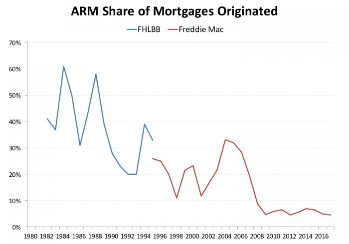
Exhibit 5 shows that shortly after regulatory approvals were provided for adjustable-rate mortgages they became a significant albeit volatile share of the market, reaching a peak of 60 percent of loans originated in the early 1980s.
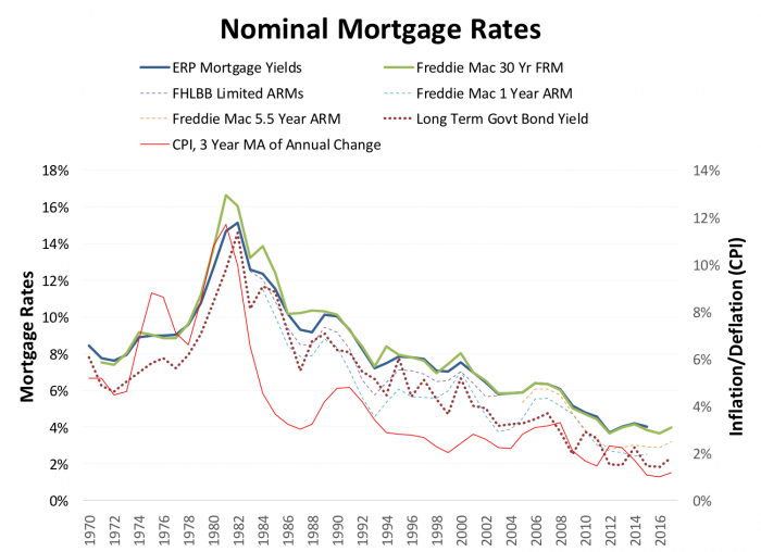
Exhibit 6 truncates the interest rate data from Exhibit 4, and adds several adjustable-rate mortgage rates. There are literally hundreds of different designs for adjustable-rate mortgages with different indexes spreads and caps. One prediction we can make is that if inflation were to increase significantly we would begin to see a return of the significant adjustable-rate mortgage market.
How Mortgage Risks Map into Different Institutions and Market Segments in the U.S.
How indeed? Economists model the main mortgage risks – default and prepayment – as complex multivariate models incorporating a number of variables representing the state of the economy (interest rates, GDP, employment, etc.), the housing market (housing prices in particular), borrower characteristics (credit score, income, debt), loan characteristics (loan-to-value ratio, fixed or adjustable rate, prepayment penalties if any, amortization schedule) and other variables including appraisal quality. We’ll keep it very simple relying on a table drawn from a study of Freddie Mac loans by Straka (2000).
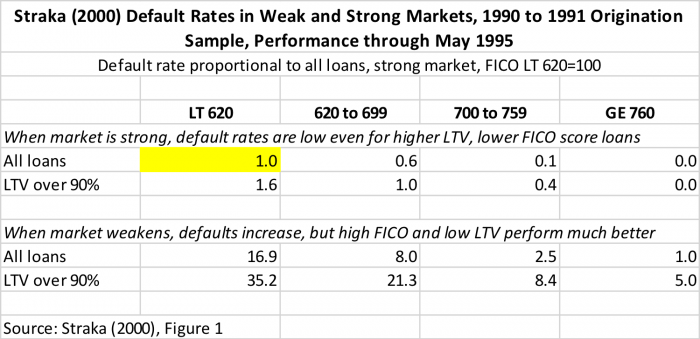
Straka’s Figure 1, which we have re-formatted as a table in Exhibit 7, presents us one representative set of results for two different sets of mortgage market conditions.
The probability of default ex ante for each combination of LTV and FICO score is normalized so that the default rate for all loans, low FICO score borrowers, in a strong regional market, is set to 1.0. Thus the probability of default, holding the economy’s condition and LTV constant, but drawing a borrower from the next higher LTV bucket, is 60 percent of the low FICO bucket. The next highest FICO bucket (700 to 759) is only 10 percent as likely to default as the low FICO bucket. In the top FICO bucket, nobody defaulted in this particular sample.
Examining the top two rows of results, and taking them at face value, there are differences by LTV and by FICO score, but they are moderate compared to what happens when we look at a weak region (not specified in detail in Straka’s article, but presumably a region with, say, high unemployment and falling house prices). In this particular sample, the low FICO borrowers default 16.9 times as often as those with the same FICO and LTV (!) And if we examine the low FICO high LTV group, they default 35 times more than the reference group.
Readers can study Exhibit 7 to get the idea. The point is not to rely on the specific results from this particular data analysis, but rather to illustrate that things like FICO score, LTV, and market conditions matter – a lot. The underwriters, if doing their jobs, will incorporate data from more sophisticated versions of Exhibit 8, to make decisions about who gets a loan and at what price. These were formerly done “by hand” i.e. with a sheet of paper and a calculator; now these are automated systems, like Fannie Mae’s Desktop Underwriter, or Freddie Mac’s Loan Prospector. With these systems, humans undertake the research that calibrates them and undertake quality control.
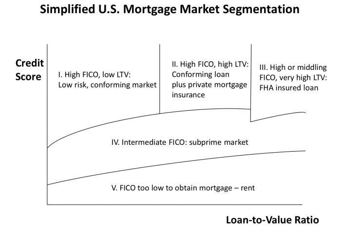
The performance we studied in Exhibit 7 leads us to Exhibit 8. Exhibit 8 presents a highly simplified diagram (an extension of that found in Cho) that explains very roughly how the U.S. mortgage market is segmented. There are many criteria for obtaining a mortgage but if we were limited to just two, we might pick credit score (FICO, for Fair, Isaac Corporation), a characteristic of the borrower, and LTV, the loan to value ratio, a characteristic of the loan. In the simplified framework of Exhibit 8, borrower characteristics, represented by FICO scores, are on the vertical axis, and loan characteristics, represented by LTV, are on the horizontal axis.
Borrowers with high credit scores can themselves be put into three categories. High credit score with a low loan-to-value ratio places us in segment I, the lowest-risk type of mortgage, often referred to as a conforming loan. In this simple diagram we abstract from the fact that past certain loan size cut-offs these will be so-called jumbo loans (i.e. above the threshold under which Congress and regulators permit the GSEs to operate). If you have a high credit score, but also a higher loan-to-value ratio (typically above 80 percent) then you still get a conforming loan, but you’ll need it take out PMI, private mortgage insurance, to cover the higher risk of default, in segment II. A very high LTV loan – say 95 percent or above –will often be insured by FHA, or the VA if one is a veteran, in segment III.
Lower quality buyers (lower FICO scores in our simple description, but in reality, underwriters also look at the level and variability of income, debt-to-income ratios, and so on) end up in the subprime market, segment IV. The subprime market itself is of course extremely complex with a number of players and many different mortgage instruments. Finally, if your FICO score is too low (or other borrower characteristics are problematic), you’ll have trouble getting a mortgage at any reasonable loan-to-value ratio and you’ll remain a renter, in segment V.
In reality there also important interactions among the independent variables that predict default. We’ve also abstracted from prepayment risk.
Of course, Exhibit 8, like Exhibit 7, is extremely simplified. Important segments of the mortgage market are omitted, including second liens, reverse mortgages, and the jumbo market for high-value loans. We haven’t specified whether the conforming market is the GSE’s (Fannie and Freddie) or private label. We haven’t said much about the details of the mortgage itself, beyond LTV; is it fixed rate or flexible? How many years is the term? How does it amortize? Are there prepayment penalties? And so on.
The lines in Exhibit 8 imply a sharp division between segments, when in the real world the boundaries are sometimes quite fuzzy. The boundary lines also shift over time and across institutions. (See the Urban Institute’s monthly Mortgage Report for one convenient summary of changing market conditions.) Substantial research has been carried out on the risks in mortgages focusing on default and prepayment which inform where those lines might be. These are, on a good day, reflected in industry practice, whether it’s adjustments to the older rules of thumb, or calibrating automated underwriting models.
The inclusion of certain neighborhood and borrower characteristics, or not, whether witting or unwitting, is itself a deep and often controversial topic. Neighborhood redlining, and discrimination against individuals by race or sex or other personal characteristics, as well as how mortgage underwriting affects affordability, are all important topics we will explore another day.
Homeownership: Have U.S. Mortgage Markets Made a Difference?
In previous posts we examined how mortgage markets and housing prices interacted; we found that credit flows drove prices more than rates did. Here we take a quick look at another variable that housing finance might affect, namely homeownership.
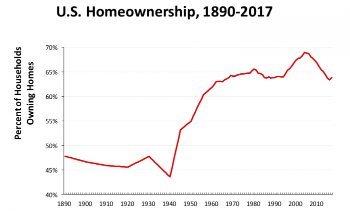
Exhibit 9 shows the dramatic increase in homeownership in the United States, especially since World War II. The percentage of homeowners has increased steadily but leveled off and even slightly declined from 1980 to 1990, then started to rise again in 1994, peaking a decade later at 69 percent. After a few years of slow decline in 2004 and 2005, the rate fell during the post-2006 collapse of the U.S. housing market, to a 2017 rate of 64 percent. For some time homeownership has been part of American politics and culture; the slight decline through part of the 1980s caused concern in some circles. It is not just mortgage terms, of course; Rajan (2010) and others have argued that some of this drop-off was probably due to a combination of demographic shifts and an increase in the user cost of owner-occupied housing relative to rental. Nevertheless, a number of additional subsidies for owner-occupied housing, especially for first-time homebuyers, have been enacted or are under consideration.
Exhibit 9 implies a large decline in the share of renters in the postwar period, which masks the fact that as the number of households in the country grew, the number of both owner and renter households grew. During the past twenty years, the number of owner households grew just under 2 percent per year, and the growth rate of renter households was almost as large. Population growth, on the other hand, was about 1 percent per year. Many new single-person households and households comprising unrelated individuals formed, so the average household size dropped from 3.2 persons in 1970 to 2.6 persons 20 years later.
Nevertheless, the idea that lending has major social effects has a strong hold on the American psyche. See, for example, the well-known film “It’s a Wonderful Life.” The movie takes place from the Depression through World War II, and its premise is that a small-town thrift institution that extends mortgage credit not only provides opportunities for homeownership and increased housing consumption, it also ensures social stability and economic growth. For a slightly more dispassionate view, see the paper by Struyk.
Where Are We Now?
The current economic context for the mortgage market is a long if slow expansion, with tighter underwriting than in the early 2000s (thank goodness), a voluminous increase in paperwork (the opposite of thank goodness), low mortgage rates if you do qualify, and low inflation. A number of signs including the Federal Reserve’s own forecasts suggest that interest rates may well be rising over the next several years, both short run and the long-run rates that are the benchmark for mortgages. However, there is no sign of the rapid inflation and high nominal rates that we saw in the 70s and 80s that created so many problems for both borrowers and lenders. We are still focused on the 30-year fixed-rate self-amortizing mortgage as the instrument of choice, although if inflation begins to pick up, nominal rates will rise, and the demand for ARMs will start to increase on the margin. Most U.S. mortgage borrowers are able to prepay and refinance without significant prepayment penalties if rates were to fall. If they do default, most mortgages do not provide recourse to lenders other than the equity which may remain in the house.
Americans also expect high LTV loans even when purchasing their first house. We’re not huge fans of saving a lot for down payments. The fixed-rate mortgage offers the borrower a one-way bet. The risk of inflation and rising interest rate are largely born by investors, unless things get so bad that taxpayers take some of the hit, as they did twice in the last 30 years.
What about other countries? Have they managed to house their population decently without the 30-year fixed-rate mortgage, without non-recourse mortgages and without a mortgage interest deduction? Stay tuned to our future post for the answer.
Sources, and Further Reading
Adelino, Manuel, Antoinette Schoar, and Felipe Severino. “Credit Supply and House Prices: Evidence from Mortgage Market Segmentation.” National Bureau of Economic Research, 2012.
Balke, Nathan S, and Robert J Gordon. “The Estimation of Prewar Gross National Product: Methodology and New Evidence.” Journal of Political Economy 97, no. 1 (1989): 38-92.
Cho, Man. “180 Years’ Evolution of the Us Mortgage Banking System: Lessons for Emerging Mortgage Markets.” International Real Estate Review 10, no. 1 (2007): 171-212.
Clapp, John M, Yongheng Deng, and Xudong An. “Unobserved Heterogeneity in Models of Competing Mortgage Termination Risks.” Real Estate Economics 34, no. 2 (2006): 243-73.
Colwell, Peter F, and Joseph W Trefzger. “Loan Underwriting Rules of Thumb.” Illinois Real Estate Letter (1995): 11-14.
Courtemanche, Charles, and Kenneth Snowden. “Repairing a Mortgage Crisis: HOLC Lending and Its Impact on Local Housing Markets.” The Journal of Economic History 71, no. 2 (2011): 307-37.
Davis, Morris A. Macroeconomics for MBAs and Masters of Finance. Cambridge University Press, 2009.
Gerardi, Kristopher, Adam Hale Shapiro, and Paul S Willen. “Decomposing the Foreclosure Crisis: House Price Depreciation Versus Bad Underwriting.” (2009).
Grebler, Leo, David M. Blank, and Louis Winnick. Capital Formation in Residential Real Estate: Trends and Prospects. Princeton University Press, 1956.
Green, Richard K. Introduction to Mortgages & Mortgage Backed Securities. Academic Press, 2013.
Green, Richard K., and Stephen Malpezzi. A Primer on U.S. Housing Markets and Housing Policy. American Real Estate and Urban Economics Association Monograph Series. Washington, D.C.: Urban Institute Press, 2003.
Green, Richard K., and Susan M. Wachter. “The American Mortgage in Historical and International Context.” Journal of Economic Perspectives 19, no. 4 (2005): 93-114.
———. “The Housing Finance Revolution.” In Susan Smith and Beverley Seale (eds.), The Blackwell Companion to the Economics of Housing. 2007.
Hartley, Leslie Poles. The Go-Between. Penguin UK reprint, 2015, 1953.
Homer, Sidney, and Richard E Sylla. A History of Interest Rates. John Wiley & Sons Inc, 2005.
LaCour-Little, Michael. “Discrimination in Mortgage Lending: A Critical Review of the Literature.” Journal of Real Estate Literature 7, no. 1 (1999): 15-50.
LaCour-Little, Michael, and Stephen Malpezzi. “Appraisal Quality and Residential Mortgage Default: Evidence from Alaska.” The Journal of Real Estate Finance and Economics 27, no. 2 (2003): 211-33.
Lea, Michael J. “Innovation and the Cost of Mortgage Credit: A Historical Perspective.” Housing Policy Debate 7, no. 1 (1996): 147-74.
Luttrell, David, Tyler Atkinson, and Harvey Rosenblum. “Assessing the Costs and Consequences of the 2007–09 Financial Crisis and Its Aftermath.” Economic Letter 8 (2013).
Malpezzi, Stephen. “Residential Real Estate in the U.S. Financial Crisis, the Great Recession, and Their Aftermath.” Taiwan Economic Review 45, no. 1 (2017): 5-56.
Mattey, Joe, and Nancy Wallace. “Housing-Price Cycles and Prepayment Rates of US Mortgage Pools.” The Journal of Real Estate Finance and Economics 23, no. 2 (2001): 161-84.
Morton, Joseph Edward. Urban Mortgage Lending. Princeton University Press, 1956.
Nichols, J, A Pennington-Cross, and A Yezer. “Borrower Self-Selection, Underwriting Costs, and Subprime Mortgage Credit Supply.” The Journal of Real Estate Finance and Economics 30, no. 2 (2005): 197-219.
Ollivaud, Patrice, and David Turner. “The Effect of the Global Financial Crisis on OECD Potential Output.” OECD Journal: Economic Studies 2014, no. 1 (2015): 41-60.
Passmore, Wayne, and Roger W Sparks. “Automated Underwriting and the Profitability of Mortgage Securitization.” Real Estate Economics 28, no. 2 (2000): 285-305.
Pedrelli, Nino Dante. “Volatility and Performance Analysis of Two Past Real Estate Markets: Mortgage Bonds of the 1920’s and Land Warrants of the 1850’s.” (2000).
Quercia, Roberto G, and Michael A Stegman. “Residential Mortgage Default: A Review of the Literature.” Journal of Housing Research 3, no. 2 (1992): 341-79.
Rachlis, Mitchell B, and Anthony MJ Yezer. “Serious Flaws in Statistical Tests for Discrimination in Mortgage Markets.” Journal of Housing Research 4, no. 2 (1993): 315.
Rajan, Raghuram G. Fault Lines: How Hidden Fractures Still Threaten the World Economy. Princeton University Press, 2010.
Rose, Jonathan D, and Kenneth A Snowden. “The New Deal and the Origins of the Modern American Real Estate Loan Contract.” Explorations in Economic History 50, no. 4 (2013): 548-66.
Roy Wenzlick & Co. Mortgage Data from Various Issues of the Real Estate Analyst, collated in Grebler, Blank and Winnick (1956).
Schwartz, Eduardo S, and Walter N Torous. “Mortgage Prepayment and Default Decisions: A Poisson Regression Approach.” Real Estate Economics 21, no. 4 (1993): 431-49.
Shiller, Robert J. “Measuring Bubble Expectations and Investor Confidence.” The Journal of Psychology and Financial Markets 1, no. 1 (2000): 49-60.
Snowden, Kenneth. “Mortgage Banking in the United States, 1870-1940.” (2013).
Straka, John W. “A Shift in the Mortgage Landscape: The 1990s Move to Automated Credit Evaluations.” Journal of Housing Research (2000): 207-32.
Struyk, Raymond J. Should Government Encourage Homeownership? Urban Institute Washington, DC, 1977.
Urban Institute Housing Finance Policy Center. “Housing Finance at a Glance: A Monthly Chartbook.” Washington, DC, 2018.